Structure refinement by the Rietveld method (Rietveld, 1969) can be carried out by EXPO2014. Graphical and computing tools are available in the program in order to attain a successful automatic or user-defined Rietveld refinement.
The refined variables include peak shape parameters, unit cell dimensions, fractional coordinates of atoms in the structure model, background coefficients, scale factor, isotropic displacement parameters. Atomic displacement parameters can be refined individually or in a group of atoms with the same atomic type or the same environment. Correction for preferred orientation can be achieved by the March-Dollase approach. The background is described using empirical functions: classical polynomial function, Chebyshev polynomial function, cosine Fourier series. The background can also modeled by mouse-click selection of pattern points. The available peak shape functions are: Pseudo-Voigt, Pearson VII, TCH pseudo-Voigt.
The non-linear least squares are carried out by employing the damped Gauss-Newton method. The refinement convergence condition is reached when the increments on parameters become smaller with respect to their standard deviations or when the relative gradient of χ2 minimized function is less then a tolerance value. Tolerance value and the maximum number of cycles could be suitably modified by the user.
The Le Bail technique can be adopted to perform a full pattern decomposition prior to Rietveld refinement in order to determine starting values of parameters (background, peak shape, zero shift and unit cell dimensions) to refine. This strategy is suggested especially if the available structure model is not completed (McCusker et al., 1999) or when the starting model is too different from the target model.
The refinement can be carried out by following two alternative approaches: 1) the user can decide the refinement strategy via graphic interface; 2) an automatic refinement schedule can be applied. In the automatic mode, groups of parameters are refined according to a fixed sequence as established in the Rietveld guidelines (Young, 1995). In the last step of refinement all parameters are refined simultaneously.
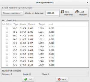
The knowledge of molecular geometry can be exploited in the refinement in form of restraints on bond distances, angles and planes. To simplify the setting of restraints, the program is able to extract from the connectivity of the initial model the possible restraints providing a list of current and target values. The user can select the restraints to be included in the refinement procedure and eventually modify the target value.
Some figures of merit are available in order to follow the progress and evaluate the quality of refinement: the weighted profile R-factor and the unweighted profile R-factor calculated for the full pattern (Rwp, Rp); the corresponding figures background-subtracted (Rwp‘, Rp‘); the statistically expected R value (Rexp); the goodness-of-fit (Rwp/Rexp); the Durbin-Watson d-statistic. R values similar to those used in case of single crystal data are also available: RF and the Bragg-intensity R which use the structure factor moduli extracted from the experimental profile.


![R_{wp}^{\prime} = \left[\frac{\displaystyle\sum_i^N{w_i(y_i-Y_{ci})^2}}{\displaystyle\sum_i^N{w_i(y_i-y_{bi})^2}}\right]^{1/2}](https://www.ba.ic.cnr.it/softwareic/expo/wp-content/ql-cache/quicklatex.com-e1bc4ef042af03e9b9398cded14731e0_l3.png "Rendered by QuickLaTeX.com")
![R_{exp} = \left[\frac{(N-P)}{\displaystyle\sum_i^N{w_iy_i^2}}\right]^{1/2}](https://www.ba.ic.cnr.it/softwareic/expo/wp-content/ql-cache/quicklatex.com-87b2f4e2626a48d3c3d6aad6cd3e3ce1_l3.png "Rendered by QuickLaTeX.com")
![\chi^{2} =\frac{\displaystyle\sum_i^N{w_i\cdot(y_{i,obs}-y_{i,calc})^2}}{N-P} = \left[\frac{R_{wp}}{R_{exp}}\right]^2](https://www.ba.ic.cnr.it/softwareic/expo/wp-content/ql-cache/quicklatex.com-8e8353c7d3ee44ae5a8226efd8dccd03_l3.png "Rendered by QuickLaTeX.com")


where N is the total number of counts in the pattern and P is the number of refined parameters.
In addition, graphical tools are available for visualizing: 1) the observed, calculated and difference pattern and the cumulative χ2 value; 2) the evolution of the structure model during the refinement in real time.
To run EXPO2014 for Rietveld refinement, first you need to create the input file. This is an example of the typical input file:
%Structure paracetamol
%Job paracetamol
%Data
Cell  7.100  9.380  11.708  90.0  97.42  90.0
SpaceGroup p 21/n
Pattern   paracetamol.xy
Wavelength 1.54056
%fragment paracetamol.cif
%rietveld
It is supposed that the cell parameters and the space group have been determined before and a structure model is available and imported by using the command %fragment followed by the file name containing the structure. %rietveld is the command to access to the Rietveld Refinement graphical interface.
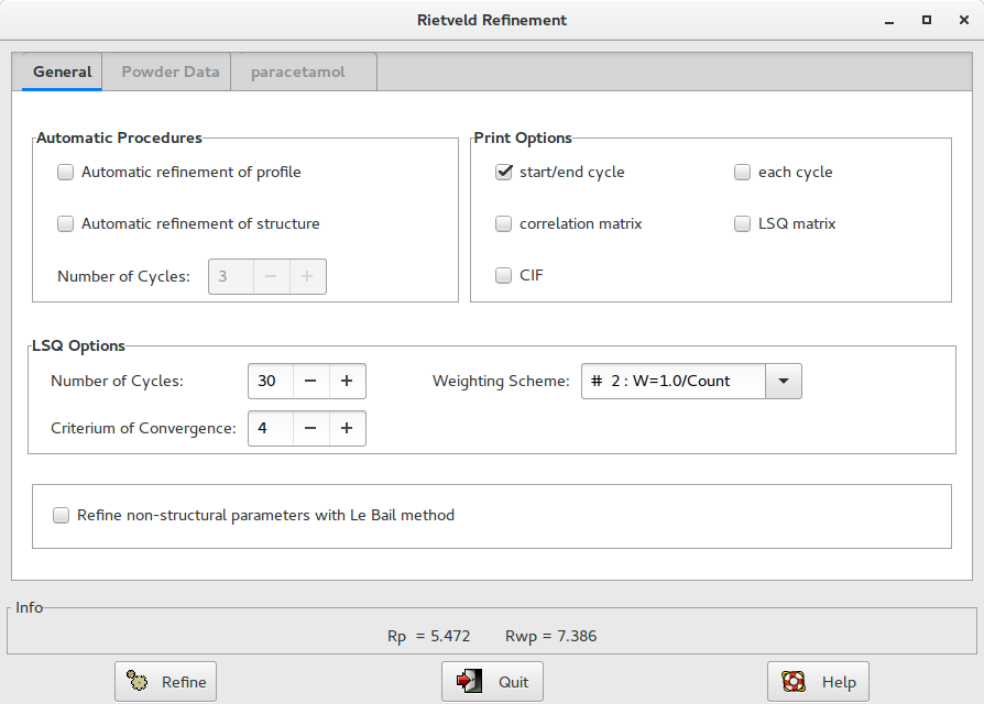
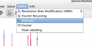
Alternatively, when a structure model is available, you can access directly to the graphic interface from menu Refine > Rietveld.
Constraints are defined as exact mathematical relationships between least squares parameters and can be used to reduce the number of parameters.
Symmetry constraints, required to conserve the space-group symmetry requirements, are mandatory and automatically deduced and imposed by the program. For example, an atom on the special position (0.5 , 0.5 , 0.5) in P-1 should not be refined at all and its parameters are constrained to these special values. Alternatively, an atom on the special position (x, x, x) in space-group P23 can be refined but must be constrained to have equal shifts applied in the x, y and z directions. Lattice symmetry establishes specific relationships between the unit cell dimensions (e.g., in cubic a=b=c and alpha=beta=gamma). EXPO2014 automatically deduces and imposes these constraints.
Constraints are often employed to control site occupancies when disorder is present in one or more sites. It is not uncommon in minerals to find an atomic site that can be occupied by either of two element types. For example, if three atoms A, B, and C occupy the same site then, assuming the full total occupancy of the site, the following relationship (or constraint) results: occA + occB + occC = 1. Thus, only two of the fractional occupancies should be refined, for example, occA and occB are free least squares variables but occC = 1 – occA – occB. Atomic displacement parameters (ADP) are made to shift synchronously. EXPO2014 automatically identifies atoms that occupy the same site and impose the constrains on site occupancies and on ADPs.
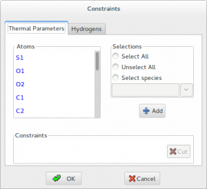
Other constraints may be imposed by the user. Clicking on the button Constraints in the Structure section under the tab with the structure name (paracetamol in figure above) is possible to access to a dialogue window to define group of ADPs that can have the same shift.
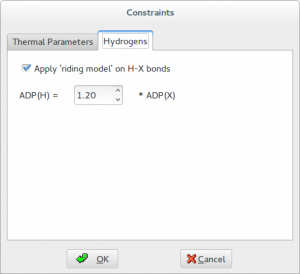
 Contraints are applied to H atoms by using the riding model. This technique is used to move H atoms synchronously with the C atoms to which they are bonded, thereby preserving the bond length and direction. The isotropic displacement parameters Uiso of the hydrogens are constrained to be 1.2 times of that of the heavy atom to which they are attached. The factor 1.2 can be changed by graphic interface.
Constraints on atomic parameters can be introduced by using the directive constr that has the following syntax:
constr constraint_equation
For example, if you want apply constraints on isotropic atomic displacement parameters use the following directive
constr B(At1) = B(At2) = B(At3) = …
in which the equation is chain of equalities. At1, At2, At3, … are the atomic labels or the order number of atoms
E.g.,
constr B(La1) = B(La2)
and the atomic displacement parameters of lanthanum atoms La1 and La2 are constrained at identical values.
The special character * can be used to specify more atoms in a constraint equation, for example, if you want apply a constraint on the displacement parameters of all 6 carbon atoms labelled C1, C2, C3, C4, C5, C6 you can write
constr B(C1) = B(C2) = B(C3) = B(C4) = B(C5) = B(C6)
or in more sintetic way
constr B(C*)
To constrain the isotropic atomic displacement parameters of all C and O atoms
constr B(C*) = B(O*)
If different atoms occupy the same crystallographic site is necessary apply a restrictions on the coordinates and on the occupation factor. Generally also the displacement parameters should be constrained.
E.g.,
constr xyz(La1) = xyz(Sn1)
constr occ(La1) + occ(Sn1) = 1
constr B(La1) = B(Sn1)
if La1 and Sn1 occupy the same site, assuming the full total occupancy of the site.
The knowledge of molecular geometry can be exploited in the refinement in form of restraints on bond distances, angles and planes. To simplify the setting of restraints, the program is able to extract from the connectivity of the initial model the possible restraints providing a list of current and target values. The user can select the restraints to be included in the refinement procedure and eventually modify the target value.
In case of structure solved by using direct space methods, bond distances and angles are generally accurate and the target value could be set equal to the current. The directive res_target_type current after the command %rietveld can be used to enable this particular setting.
Rietveld, H.M. (1969). J. Appl. Cryst. 2 65–71.
McCusker, L.B.; Von Dreele, R.B.; Cox, D.E.; Louër, D.; Scardi, P. (1999). J. Appl. Cryst. 32, 36-50.
The Rietveld Method. Edited by R. A. Young, Oxford University Press, Oxford (1995).