THE GRAPHICAL USER INTERFACE

Start the RootProf GUI by typing on the ROOT promp:

root> .x RootProfGui.C

the following graphical window will appear on your terminal:

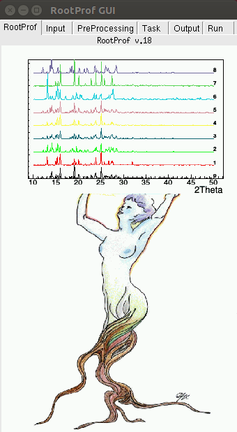
Here you can prepare the command file from the pages Input, PreProcessing, Task, Output. From the page Run you can check the command file prepared by the GUI and run RootProf on it. You can also run RootProf on a command file prepared previously.

To start preparing the command file go to the page Input of the RootProf GUI. The following graphical window will be shown:

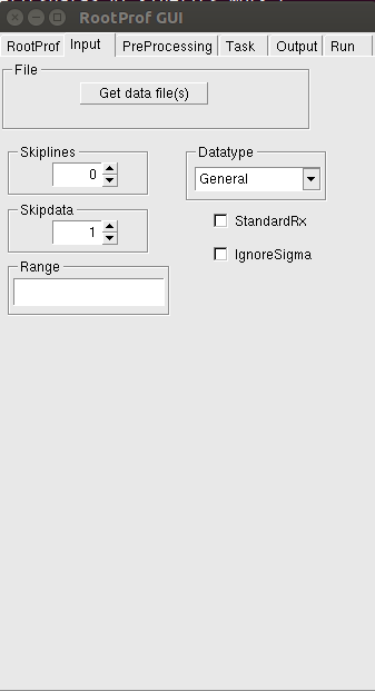
Please refer to the General Commands page to know the meaning of the commands. Tooltip windows will appear on some of the boxes when you pauses the mouse pointer over them, to further explain the meaning of the command. You can check each individual click on the GUI, since the corresponding command added to the command file appears on the terminal.

The values defining the range of the independent variable to be used for the profiles loaded should be written in the Range box (see description of the command Range in the General Commands page).

By clicking the Get data file(s) button the following window will appear:

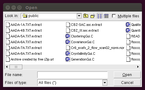
From it you can load the data files. Individual profiles can be loaded one by one, or all together, by checking the Multiple files button.  As an alternative, a data matrix containing a set of profiles can be loaded as a single file.

Use the Datatype menu to set the Datatype command corresponding to the data files loaded.

Use the Range box to restrict the analysis to a range of values. More ranges can be defined, to skip unwanted regions of the profiles.

The Preprocessing page allows to set the proper preprocessing, to be applied to each profile loaded.

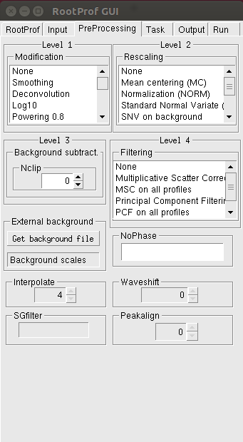
Here four level of preprocessing can be set, operating independently one after the other: Modification (level 1), Rescaling (level 2), Background subtraction (level 3) and filtering (level 4). Several options for each level of preprocessing are available (see description of the command Preprocess in the General Commands page). Nclip is the size of the clipping window for background subtraction. To generate the Preprocess command in the command file the options in the Level 1, Level 2 and Level 4 boxes must be selected.

The Get background file button can be used to load an external background file (for example an empty target measurement). The scale factors that have to be applied to subtract this background to each data file should be given in the Background scales box (the number of scale factors should be equal to the number of data files). See description of command Backscale in the General Commands page.

The minimum and maximum values of the independent variable that enclose the peaks to be cancelled from the profiles (see description of the command Nophase in the General Commands page) should be written in the NoPhase box.

The Interpolate, Waveshift and SFfilter boxes are activated upon selection of the Interpolation, Waveshift and SG filtering Level 1 preprocessing, respectively. The Peakalign box is activated upon selection of the Peak alignment Level 4 preprocessing.

The analysis to be done on data files is chosen by using the Task page.

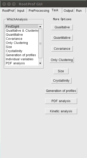
For a detailed description of different analysis see the command Whichanalysis in the General Commands page. More options are needed in case of specific analyses, which can be set by clicking on the respective buttons. For example, additional options for Qualitative analysis can be set from the following window:

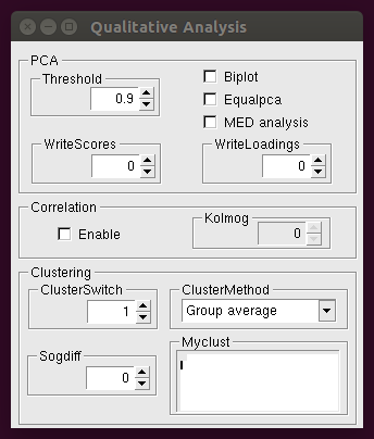
Detailed description of corresponding parameters can be found in the Qualitative Analysis page.

The values defining the range of the independent variable to be used for the profiles loaded should be written in the Range box (see description of the command Range in the General Commands page). The box Myclust is an editor window. Here you can insert Myclust commands according to what described in the General Commands page, and then save the changes by clicking with the right mouse button and selecting Save from the menu. Please consider that the Myclust editor is activated only if ClusterSwitch is set to 2.

The following window appears after clicking the Quantitative button:

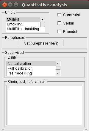
A detailed description of these parameters can be found in the Quantitative Analysis page. The boxes Rhoin, test, referw and Msa are editor windows. Here you can add text and then save the changes by clicking with the right mouse button and selecting Save from the menu. This can be also done by using the Command file editor available in the Run page.

The following window appears after clicking the Covariance button:

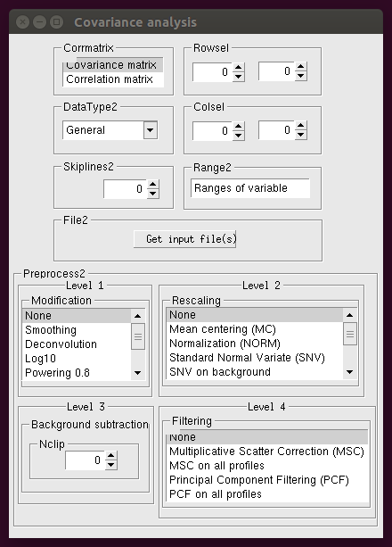
A detailed description of these parameters can be found in the Covariance Analysis page. To generate the Preprocess2 command in the command file the options in the Level 1, Level 2 and Level 4 boxes must be selected.

The following window appears after clicking the Only Clustering button:

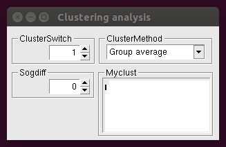
where the parameters driving hierarchic clustering of profiles (see the Qualitative Analysis page for a detailed description) can be set. They are applied to a distance matrix given as data file. This window is also useful to carry out the analysis of the distribution of individual variables of the profile (whichanalysis 11), since it allows to set up the myclust definitions.

The following window appears after clicking the Size button:

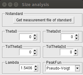
A detailed description of these parameters can be found in the Size Analysis page.

The following window appears after clicking the Crystallinity button:

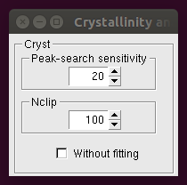
The first two boxes refer to a calculation based on a fitting procedure (see the Crystallinity Analysis page for a detailed description of these parameters). If the Without fitting button is checked, a different calculation is performed, where the crystallinity is calculated by considering the intensity counts after a background subtraction step.

The following window appears after clicking the Generation of profiles button:

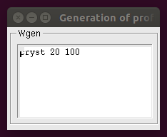
where the editor of the Wgen box can be used to write linear coefficients for profile generation though the command wgen (see description of the command wgen in the General Commands page).  The command is followed by a series of numbers comprised in the range [0,1]. They should be as many as the number of profiles loaded with the command file. The changes done in the editor window can be then saved by clicking with the right mouse button and selecting Save from the menu.

The following window appears after clicking the PDF analysis button:

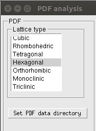
The type of lattice guessed for the PDF profile can be set from the Latttice type box. In case of dimetric cell (Tetragonal or Hexagonal lattice) or trimetric cell (Orthorhombic, Moniclinic, Triclinic lattice) the Set PDF data directory button is enabled. It can be used to set your local directory where the pre-calculated PDF data, supplied when downloading RootProf, are stored. See the PDF Analysis page for a detailed description of these parameters.

The following window appears after clicking the Kinetic analysis button:

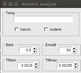
The temperature values corresponding to each line of the file read in input should be written in the Temp box. See the Kinetic Analysis page for a detailed description of these other parameters.

Options related to the text and graphical output are set by using the Output page.

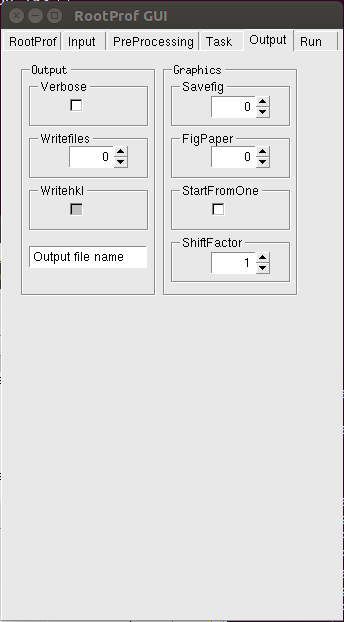
where the name of the output file to be used to redirect text output has to be written replacing the writing "Output file name". For an explanation of the commands please refer to the General Commands page.

RootProf can be executed by using the Run page.

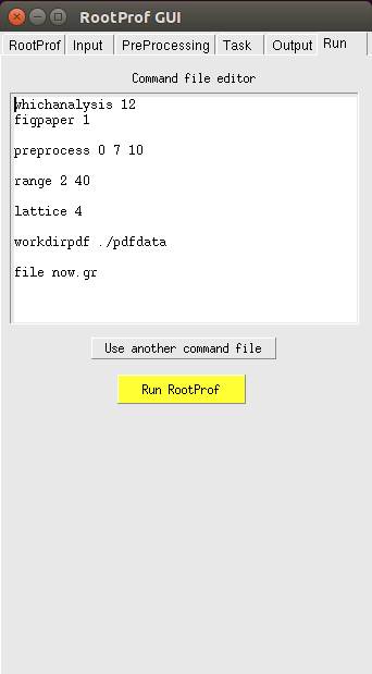
where the Command file editor shown the commands written in the command file. You can eventually change the command file within the editor window. Changes can be saved by clicking with the right mouse button and selecting Save from the menu.

Just click on the yellow button to run RootProf with this command file. You can also run RootProf by using another existing command file by selecting this file with the button "Use another command file". The command file loaded will appear on the Command file editor, so that you can check it and modify it before running RootProf.

NOTE:

When RootProf ends its execution, the promt

root>

will appear on the ROOT terminal window. Then you can play with the graphic windows. If you want to execute again RootProf, you should first close the ROOT session with the command:

root> .q

and then run again ROOT and RootProfGUI.