Direct space methods for crystal structure determination from powder diffraction data have become widely available and popular in recent years and have successfully been applied to solve the structures of organic, inorganic and organometallic materials. Different but similar procedures can be realized: grid search, Monte Carlo, simulated annealing (SA), parallel tempering, genetic algorithm, particle swarm. Each method involves the generation of a random sequence of trial structures starting from an appropriate 3D model and moving it until a good match between the calculated and the observed pattern is found. The information about chemical knowledge of molecules is actively used to reduce the number of parameters to be varied: bond distances, bond angles and ring conformation are usually known and kept fixed while only the torsion angles are varied during the procedure.
Two Direct Space algorithms are available in the EXPO2014 program, for crystal structure solution.
They are: 1) a classical Simulated Annealing (SA) approach; 2) the Hybrid Big Bang Big Crunch (HBB-BC) algorithm (Altomare et al., 2013). It results from an appropriate combination of BB-BC approach with SA and relies on one of the evolutionary theory of the universe consisting of two successive phases: 1) the Big Bang, corresponding to an energy dissipation procedure for creating a completely random initial population; 2) the Big Crunch, corresponding to a contraction procedure for converging to a global optimum point. This procedure is automatically applied by the program for compounds described by less than 6 internal degrees of freedom (torsion angles) and constituted by less than 3 fragments. In all the other cases the classical SA approach is used.
To perform EXPO for structure solution using direct space methods, you’ll first need to create an input file. It’s assumed that the cell parameters and space group have already been determined.
The example input file, paracetamol.exp, is shown below. You can use this file for the structure solution of paracetamol using simulated annealing within EXPO.
%Structure paracetamol
%Job paracetamol
%Data
        Cell  7.100  9.380  11.708  90.0  97.42  90.0
        SpaceGroup p 21/n
        Pattern   paracetamol.xy
        Wavelength 1.54056
 %fragment paracetamol.mol
 %sannel
You can import this file by going to File > Load & GO in the main menu. The file paracetamol.exp is already located in the example folder.

%sannel is a command to access to the Simulated Annealing graphic interface.
%fragment paracetamol.mol is the command to import the starting structural model for Simulated Annealing in MDL Molfile format (*.mol). This command can be repeated several times to import more than one fragment (see the section Usage of command %fragment). Some other file types can be imported in the same way: MOPAC file (*.mop), Tripos Sybyl file (*.mol2,*.ml2), C.I.F. file (*.cif), Protein Data Bank file (*.pdb), Fenske-Hall Z-matrix (*.zmt), EXPO fragment or Free Fractional Format (*.frac), XYZ format (*.xyz), Tripos SYBYL (*.mol2, *.ml2), Shelx File (*.ins, *.res). A complete list of the supported input file can be find in section Import of this document.
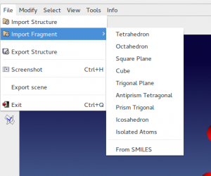
Instead of command %fragment name_starting_model.ext, with ext=mol, frac, cif etc, you can import the starting structural model directly by the graphic interface from the menu File > Import.
Modify > Add fragments to add fragment to an existing partial structural model.
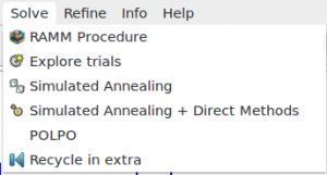
Instead of command %sannel, you can access directly to the graphic interface from menu Solve > Simulated Annealing.
Press the button ![]() in the dialog window to run the Simulated Annealing procedure.
in the dialog window to run the Simulated Annealing procedure.
The required starting model can be described in terms of combination of scattering objects that are molecular fragments e.g., isolated atoms, molecules, coordination polyhedra. For each molecular fragment, the position may be defined by the fractional coordinates (x, y, z) of the center-of-mass or a predefined pivot atom, the orientation may be defined by rotation angles (θ, φ, χ) around a set of orthogonal axes, and the intramolecular geometry may be specified by a set of n variable torsion angles {τ1, τ2, …, τn}. These concepts may be extended to the case of two or more (identical or nonidentical) molecular fragments within the asymmetric unit (a.u.). In general bond lengths, bond angles and ring conformation are not considered as variables during the optimization procedure, but they should match as closely as possible that of the studied compound. One of the drawbacks of global optimization methods is to input an accurate 3D starting structural model of the a.u.
Starting model for direct-space method can be prepared by the following two strategies, or by a combination of both approaches.
1) The user is strongly advised to check for similar molecules in the Cambridge Structure Database (CSD) (organics & organometallics) or in the Inorganic Crystal Structure Database (ICSD) (inorganics, elements, minerals & intermetallics) or in the Crystallography Open Database (COD: http://www.crystallography.net/) or in the crystallographic literature. If a new structure is being studied, one can frequently find significant molecular parts of the structure in existing crystal structures. Molecular fragment found in database can be modified and optimized by quantum-chemistry package to finally generate the desired structure.
Some open chemistry database where look up molecules are:
- NIST Chemistry WebBook: http://webbook.nist.gov/chemistry/
- PubChem: https://pubchem.ncbi.nlm.nih.gov/
- Drugbank: http://www.drugbank.ca/
Calculated 3D molecules in sdf, pdb, mol format can be find in these database and imported in EXPO2014. Computed Simplified Molecular-Input Line-Entry System (SMILES), when available, can be converted in 3D molecule by File > Import Fragment > From SMILES or Modify > Add Fragments > From SMILES. You can verify that the bond lengths have reasonable values using a tables of standard bond lengths available in Volume C of International Tables for X-Ray Crystallography.
2) Starting molecular model can be created by geometry optimization using quantum-chemistry package, e.g., MOPAC, Gaussian, Gamess, NWChem, etc. Nowadays this is usually done by building the molecule with an interactive builder in a graphical user interface, then optimizing it with forcefield method with the click of mouse. The resulting structure is then subjected to an ab initio, semi-empirical, or DFT calculations.
Some free available software that can be used to sketch molecules, optimize the geometry by forcefield method and create input file for the quantum-chemistry calculations are:
- Avogadro: http://avogadro.cc/wiki/Main_Page
- Gabedit: http://gabedit.sourceforge.net/
- ACD/ChemSketch: http://www.acdlabs.com/resources/freeware/chemsketch/
- MarvinSketch: https://www.chemaxon.com/products/marvin/marvinsketch/
See the section Geometry Optimization for more information about the support provided by EXPO2014 for theoretical calculations.
The description of crystal structure is straightforward in the case of molecular organic crystals: isolated molecules with known chemical connectivity are packed together by weak intermolecular forces. Because the starting model should be a tridimensional representation of the a.u., is important to known how many molecules are contained in the a.u. (Z’). In case of molecular compounds the a.u. is usually a molecule or occasionally two or more molecules which differ from one another in orientation or conformation (Z’>1). When a molecule posses symmetry coincident with a crystallographic symmetry element, it may occupy a special position, and the a.u. will then be a half molecule or even some smaller fraction (Z’<1). Inorganic materials often consist of connected polyhedra and the topology of this connectivity is not generally known a priori and thus building a model of inorganic crystal structure for global optimization is often less straightforward and clear. Software provides tool to import some regular polyhedra or you can find the type of polyhedra you need from literature or from database. The choice of the number of each polyhedra to use must be made, talking into account how many atoms are expected per unit cell (volume of atom in the cell). These non‐molecular crystals usually crystallize with higher symmetries, and atoms often occupy special positions. At the same time it is necessary to take into account the possibility that polyhedra share atoms at the corners. The use of dynamical occupancy correction (DOC) is able to automatically correct the occupancy of atoms if they are close to a special position or in case of overlap between atoms of the same atomic type. DOC could be very useful when the exact composition of the studied compound is a priori not known exactly. Theoretically this means that it is possible to add more atoms than initially deemed necessary, expecting the DOC to artificially merge the excess atoms. It is also possible to solve structures putting into the cell independent atoms at random positions, but the observation/parameter ratio (‘observation’ here means the number of reflections) should be at least 8 or more depending on the quality of diffraction data.
The dialog window of Direct Space algorithms in EXPO2014 is composed by 4 pages.
The first page contains the general settings of Simulated Annealing algorithm:
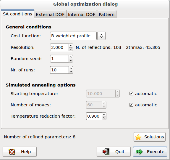
Cost function: 2 cost functions can be selected: R weighted profile ( ), R-Bragg intensities (
 ). 1.The default cost function is , which is the agreement factor usually used in the Rietveld refinement

where  and
and  are the observed and calculated profile values at the
  value of the i-th experimental step, respectively, and
  . If is used there is no need to extract the structure factor moduli and a profile fitting procedure must be carried out. This task is automatically performed by EXPO2014 before starting SA.
2. factor that compares the experimental integrated intensities  with the intensities
  calculated by the model

The preliminary extraction of experimental integrated intensities is automatically performed by EXPO2014 by using the Le Bail algorithm, before starting SA. The advantage of using with respect to is that it offers a significant reduction of the computational time, but, if the overlap is severe, can be unreliable because the values can be affected by large errors.
Resolution: defines the maximum resolution used by Simulated Annealing procedure. Direct space methods do not require the use of the entire pattern: usually the algorithm works well with data up to 2 Å resolution.
Random seed: selects the value determining the sequence of random numbers used from the algorithm. When is set to 0 the random seed will be calculated by the system clock.
Nr. of runs: select the number of Simulated Annealing runs. At the beginning of each run a new value of random seed is calculated.
Starting temperature: selects the starting temperature. Check on ‘automatic’ and the program automatically will find the starting temperature at the beginning of the procedure.
Number of cycles: the number of moves for each step of temperature is Np*N*20 where Np is the number of refined parameters and N is a number set by the user in the entry box. Choosing ‘automatic’ the program automatically will determine the value of N by taking into account the external and internal DOFs and the flexibility of the molecule. This number can be modified also by directive niter (see above).
Temperature reduction factor: the reduction factor applied to the temperature at each step in the annealing schedule. The default value is 0.90. Increasing this value, the chance to find the global minimum can be improved even if a longer execution time will be taken by the procedure.
Solutions: browse the best solutions saved at the end of each run.
The second page External DOF contains information about the external degrees of freedom (DOFs):
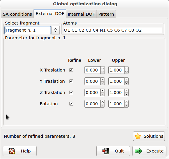 Select fragment: selects the fragment and visualizes the corresponding structure information. Atoms: list of the atoms in the selected fragment. Parameter for fragment: list of the external DOFs for the selected fragment. Check the parameters to refine, enter the lower and upper bounds of the parameters.
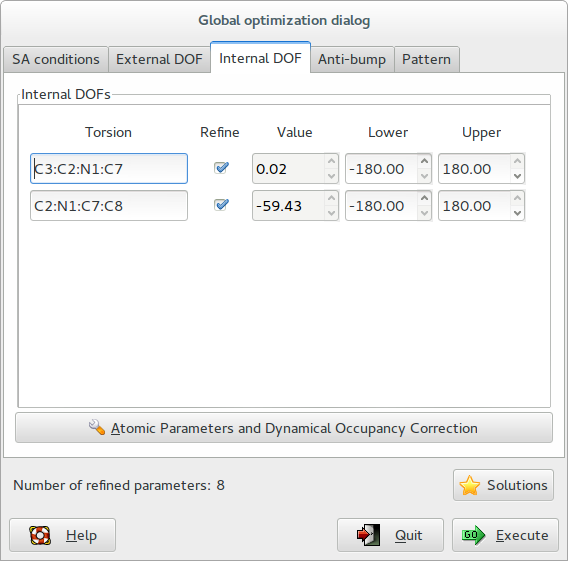
The third page Internal DOF contains information about the internal degrees of freedom (DOFS):
Internal DOFs: list of the torsions associated to each refinable internal DOF. Check the parameters to refine, enter the lower and upper bounds of parameters.
Press the button ‘Atomic parameters and Dynamical Occupancy Correction’ to access to the following dialog window:
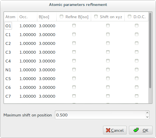
Thermal parameters: check the buttons on column ‘B[iso]‘ to refine the thermal parameters of atoms. Click on label ‘B[iso]‘ to select all checks in the column. If the thermal parameters are not indicated in the imported fragment file, the program assigns the default values of B=3.0 for non-hydrogen atoms and B=6.0 for hydrogen atoms. These default values can be changed editing the new values in the column. The refinement of the thermal parameters is discouraged because usually doesn’t improve the results.
X Y Z: check the buttons on column ‘Shift on xyz’ to refine the atom positions, in this case the fragment is not rigid but the atom positions are shifted respect to the barycentre. Click on label ‘Shift on syz’ to select all checks in the column. The positions refinement (x,y,z) is generally discouraged because can considerably increase the time to reach the global minimum.
Maximum shift on position: enter the value of the maximum shift of the atomic positions. 0.020 is the suggested value. Increasing this value the explored parameter space becomes wider so increasing the probability of falling into a local minimum.
Dynamical Occupancy Correction (DOC): automatic detection of atoms in special position and atoms that share the same position. If this option is not active all refined atoms are considered in general position (default). DOC will be applied only on the atoms selected in the column D.O.C., select all atoms if you don’t know exactly which atoms will fall into special positions. DOC slows down the computation time so it should be avoid if non special position or shared atoms are expected
Pattern: Enter the direction of the preferred orientation and check ‘G Factor’. The March-Dollase correction will be applied and the magnitude of the preferred orientation will be optimized.
A visual match between observed and calculated powder pattern is plotted when Simulated Annealing is running, the progress of structure solution is monitored and the user can examine: 1) the graph of the minimum values of the cost function (CF) vs. the number of moves; 3) the crystal packing by using the button ![]() on the JAV viewer.
on the JAV viewer.
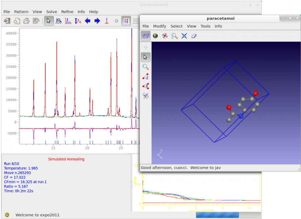
During the Direct Space runs, three buttons are active on the toolbar of the main window: ![]() opens the JAV viewer for crystal structure visualization.
opens the JAV viewer for crystal structure visualization. ![]() skips the current run.
skips the current run. ![]() stops the procedure.
stops the procedure.
When the quantity of information available from a powder diffraction pattern is limited (due to, e.g., severe peak overlap, broad peaks, preferred orientation, presence of weak scatters) and/or the number of degrees of freedom is large, it may be necessary to add extra chemical information to the optimization process in order to obtain the correct solution. In fact, in this situation, the correct structure may not correspond to the minimum of CF. The use of restraints on bond distances and angles or the application of bond valence restraints are approaches to increase the probability to obtain only chemically plausible models (Falcioni & Deem, 1999; Favre-Nicolin & Černỳ, 2002). In particular if the final global solution contains atoms colliding each other, anti-bumping restraints can be used to avoid this solution. They are relationships between atoms to prevent atomic group overlapping with other parts of structure. The restraint can be implemented as normal distance restraint, which is only applied if the interatomic distance becomes less than some threshold. The contribution of the anti-bumping restraints to the global cost function is measured by the espression

with the condition  , where
  and
and  are the minimum ideal distances and the model distances, respectively, between pairs of atoms
  and
and  , and summation is over
  contacts,
  is equal to 2 (Hendrickson, 1985). depends on the atomic elements in contact and on the type of contact, in particular if the two atoms are hydrogen-bonded atom pairs. in default are defined as the sum of the atomic radii of the two atoms multiplied by a scale factor
  (0.7 is the default value)

and  and
and  are the van der Waals radii (Feng et al., 2009). This minimum distance can also be modified by the user for each pair of atom types by using the directive bump. The directive bscale allows the modification of the scale factor on distances (o.7 is the default value). Increase if the default value is not able to avoid structures with overlapped atoms.
  is recommended value. Small value of (e.g.,
  ) are recommended if the anti-bumping restraints are applied between isolated atoms in the starting model but that are expected to be connected in the final structure. In principle, the weight
  associated to restrains varies with the type of restrains, but in practice a uniform value is used (1.0 is the default value). You could change this value.
Use the directives bump and/or nobump if you are interested in applying restraints between specific atoms and to between groups of atoms of the same species. The weight and scale factor can be modified by using the directives bweight and bscale.
Output file contains a list of all applied anti-bumping restraints with the distances and .
All pairs of atoms separated by a rigid sequence of bonds (e.g., two atoms in a rings) are excluded from the anti-bumping interactions. In case of intramolecular contacts it is also advantageous to exclude atoms that are separated by a short contiguous flexible chain of covalent bonds. The applied rule consists to exclude all atoms that are separated by a path of bonds containing 4 rotable bonds or less.
The application of restraints is relatively time-consuming because requires that all symmetry equivalent atoms are taken into account. Strictly speaking, it should be unnecessary and it should be use only when the quality of the diffraction pattern is insufficient to avoid that the final solution contains overlapping atoms.
Bond valence sums can be introduced as restraints in the optimization process adding to the  sum another term with the form:

where the sum is done over  bond valence restraints,
  is a suitable weight assigned to each restraint,
  is the bond valence sum of an atom with the expected formal charge
  . The directives bvres and bvpar are available to set bond valence restraints.
The output file generated from the procedure, contains information on:
- Starting crystal structure
- Volume per atom
- Connectivity
- Internal and external DOFs
- List of restraints
- List of optimized parameters
- Each SA or HBB—BC run
- Summary of all the SA or HBB—BC runs
- The selected final structures at the end of each run the structure coordinates are saved in CIF file with name created by project name with suffix _best1, _best2, (e.g., paracetamol_best1.cif is the best solution, paracetamo1_best2.cif is the second best solution, etc.). The order number in the name represents the position in the list of structures ordered according to the cost function.
When Direct Space approaches fail:
1) The default conditions, in particular for complex structure, could not be appropriate. Increase ‘Number of moves’ and ‘Nr. of runs’ in the tab ‘SA conditions‘, these are the most important parameters in determining the success of the optimization process. You can double or, if necessary, triple the default value of ‘Number of moves’ to be sure to find the global minimum. The directives niter and nrun can be used to set these parameters directly in the .exp input file. Some examples about the application to complex problems are reported at this link.
2) The quality of data is not good and the diffraction pattern is not suitable for the extraction of the integrated intensities. In this case can be convenient to perform the optimization by using the R weighted profile cost function.
3) The starting model is incorrect: bond distances and angles are not entirely accurate, the number of building blocks is wrong. Improve your model with Cambridge Structural Database (CSD) or building packages (Avogadro, ChemSketch, ChemDraw, …), check the volume per atom in the output file (about 15-20 Ang/atom).
4) The assumption about thermal factors is invalid. Check thermal factors from similar structures and/or include them in the optimization process by the window dialog ‘Atomic parameters and dynamical Occupancy Correction‘. See also the directive refinetf.
5) Space group and cell parameters are not correct. Additionally, in many cases it may be necessary to carry out a series of independent calculations to test different potential space groups and/or unit cell choices.
Usually you don’t need to read this paragraph unless you are interested to run Simulated Annealing without interaction with graphic interface. In this case use the command %sannel to run Simulated Annealing from the input file (*.exp). Use command %automatic to skip the interaction with the graphical interface and the program will perform the Simulated Annealing using the default values. An example of input file with command %automatic and %sannel is the following:
%automatic
%Structure paracetamol
%Job paracetamol
%Data
        Cell  7.100  9.380  11.708  90.0  97.42  90.0
        SpaceGroup p 21/n
        Pattern   paracetamol.xy
        Wavelength 1.54056
%fragment paracetamol.mol
%sannel
To modify the default values of SA, some directives can be used after the command %sannel in the .exp input file.
An example of application of directive niter and nrun to increase the percentage of success in case of structure solution of the largely flexible molecule verapamil hydrochloride
%Structure verapamil
%Job Verapamil hydrochloride (C27H39N2O4.Cl)
%Data
        Cell   7.089  10.593  19.207  100.11  93.75  101.56
        SpaceGroup p -1
        Pattern    verapamil_hydrochloride.xy
        Wavelength 1.54056
%fragment verapamil_hydrochloride.mol
%sannel
       niter 2000
       nrun 20
The following directives must be added after the command %sannel in the input file to activate some specific features of the simulated annealing procedure
Abbreviations for directives name at least 4 character are permissible, i.e. cost 2 instead of cost_function 2.
bump
or
bump atoms1 atoms2 [dist wei]
bump directive is used for the generation of anti-bumping restraints. If this directive is used without additional parameters anti-bumping restraints are automatically generated and extended to all C, N, O and S atoms. The atoms1 and atoms2 parameters must be used to apply restraints between specific atoms or between groups of atoms of the same species. atoms1 and atoms2 are the label of atom. If S is an atomic specie, the symbol S* should be used to refer to all the atoms of the same species. The special symbol * select all atoms. Use frag1, frag2, … to refer to entire molecular fragment. dist and wei are optional parameters. dist can be used to specify the minimum distance at which the restraint is active. wei is the weight associated to the restraint. Negative values of dist and wei will be ignored applying the default values that are: sum of Van der Waals radii for dist, 1.0 for wei. Complete list of generated anti-bumping restraints is available in the output file.
E.g.
bump
anti-bumping restraints are applied only to all C,N,O,S atoms in the structure
bump C* S*
apply anti-bumping restraints only between C and S atoms. Default values are assigned to dist and wei.
bump C1 S1 3.5 10.
apply anti-bumping restraint only between C1 and S1 atoms
bump C* S1 -1 10.
generate anti-bumping restraints between all C atoms and the S1 atom. The weight is set to 10. and the default value is used for distance.
bump C1 S1 3.5 10.
bump C1 C2 -1 10.
bump directives can be combined to generate specific restraints lists.
bump
bump C1 S* -1 10.
anti-bumping restraints are applied only to all C,N,O,S atoms in the structure. The weight for contact between C1 and all sulfur atoms is set to 10.
bump C1 *
generate anti-bumping restraints between atom C1 and all other atoms.
bump frag1 frag2 -1 10.
generate anti-bumping restraints between the atoms in the molecular fragment 1 and the atoms in the molecular fragment 2.
nobump atomsl atoms2
Delete anti—bumping restraints. This directive makes sense if applied in combination with bump directive to remove previously set restraints.
E.g.
bump * *
nobump Ag1 N1
nobump Ag1 N2
This combination of 3 directives generates anti-bumping between all atoms except between atom Ag1 and N1, Ag2 and N2.
bump
nobump O5 *
This combination of 2 directives generates anti-bumping between all O,C,N,S atoms except O5 oxygen atom.
bweight w
This directive controls the weight on all anti-bumping restraints. The default weight is 1.0.
bscale s
This directive allows the modification of the scale factor applied to a sum of Van der Waals radii in the definition of the default minimum distance between two atoms for anti-bumping restraints. 0.7 is the default value. If you increase this value, you increase the minimum distance and the number of contacts that contribute to the cost function.
cost_function n
To choose the cost function: 1 for Rw-profile, 2 for RF, 3 for RI. The default choice is 1.
doc
or
doc atom1 atom2 atom3 …
Activate the dynamical occupancy correction (DOC). By default DOC is applied to all the atoms unless you specify a list of atoms.
E.g.
doc Ni1
DOC will be applied only to the atom Ni1.
centre_of_rotation atc
or
centre_of_rotation atc atf
This directive is used to specify the origin of rotation. atc is the label of the atom chosen as centre of rotation and the rotation will be applied to the molecular fragment containing the atc atom. A second generic atom atf included in the molecular fragment may be indicated when the centre of rotation atc is not a part of the fragment. As default choice, the centre of rotation is the central atom in case of polyhedra; the center of rotation is the center of mass for all other type of scattering objects. The keyword @com can be used to change the default choice in case polyhedra. The origin of rotation for each molecular fragments is reported in the output file in the section ‘List of fragments’.
E.g.
centre_of_rotation P1
The atom P1 is the origin of rotation of the molecule P(C6H5)3 containing P1
centre_of_rotation Ni1 P1
The molecule P(C6H5)3 containing the atom P1 will be rotated around Ni1
centre_of_rotation @com Si1
The polyhedron containing the Si1 atom will be rotated around the center of mass. This directive modify the default choice of program.
export ncif
This directive is used to specify the number of CIF files (ncif) to generate at the end of the optimization procedure.
E.g.
%sanneal
nrun 100
export 5
Only the best 5 solutions out of 100 runs will be saved in a cif file.
extdof atom [translation_code rotation_code]
To fix external DOFs of a specific molecular fragment. atom is any atom belonging to the molecular fragment. translation_code and rotation_code must be 0 to fix the translation and rotation respectively and 1 to refine it. The default is 1.
E.g.
extdof Si1 0 0
Translation and rotation parameters of the molecular fragment containing the Si1 atom will be not optimised.
intdof atom optim_code
or
intdof atom1 atom2 [optim_code]
To fix the optimization of a specific internal DOF. This directive can be used in two different ways.
a) To select all the internal DOFs of a molecular fragment where atom is any atom in the fragment.
b) To select a specific internal DOF. In this case atom1 and atom2 must be the 2 atoms that define the rotation axis. This directive is useful when, relying on the prior chemical knowledge of the structure, some internal DOFs can be fixed, for example double bonds.
optim_code must be 0 to fix and 1 to enable the optimization. The default is 1.
E.g.
intdof C1 C2 0
Fix the internal DOF corresponding to the rotation around the C1-C2 axis.
intdof C1 0
Fix all internal DOFs of the molecular fragment containing the C1 atom.
extdof Si1 0 0
intdof Si1 0
intdof is used in combination with extdof directive to fix an entire framework of silicon atoms.
intdof_disp atom1 atom2 atom3 atom4 disp [mode]
These directive can be used to apply a specific displacement to the rotation associated to the torsion atom1-atom2-atom3-atom4. atom1, atom2, atom3, atom4 are the atoms that define a specific torsion. The torsion will be sampled in the interval  where
where  is the initial value of the torsion.
mode is an optional parameter that can be used to specify whether the torsion is bimodal (mode=2) or trimodal (mode=3), default is mode=1. This information can be very useful in case of expected bimodal planar torsion ( ); for example, if disp is equal to 30°, the torsion will be sampled in two range if mode=2 is specified:
  and the complementary range
  .
.
If the torsion is not planar and the starting value is 60°, the sampling ranges will be:  and
and  . In case of trimodal torsion, 3 ranges will be sampled: the range around the starting value and two additional range at +120° and -120°.
E.g.
intdof_disp N1 C2 C2 B2 30
The directive is used to limit the sampling of the specified torsion.
intdof_disp C1 C2 C3 C4 20 2
The torsion C1-C2-C3-C4 is expected to be bimodal and planar. The starting value of the torsion must be zero or close to zero.
move atom1 @(x y z)
The move directive can be used to move the position of a molecular fragment in a specific position.
atom1 is the label of an atom contained in the molecular fragment and x y z are the final fractional coordinates of atom1 after translation of the entire fragment.
This directive can be useful when a position of an atom is already known, for example an heavy atom located by direct methods.
E.g.
move Ni1 @(0.5 0.286 0.75)
extdof Ni1 0 1
centre_of_rotation Ni1
The move directive is used to move the molecular fragment with Ni1 to a specific position. The combination of the directives extdof and centre_of_rotation activates the rotation around Ni1 fixing the translation.
niter n
To modify the number of moves for each temperature step. In a default run the number of moves is automatically calculated. This parameter is important in determining the success percentage of the optimization procedure.
nrun n
To modify the number of simulated annealing runs. The default is 10.
resmax val
To define the maximum resolution used by simulated annealing. The default value is 2.0 Å.
temper temp
To modify the initial temperature. In a default run the initial temperature is automatically calculated.
tfactor val
Determines the temperature reduction factor. val ranges between 0 and 1 and its default value is 0.90.
optimadp overall
optimadp species
optimadp molecules
optimadp atoms atoml atom2 atom3 …
optimadp groups atoml atom2 atom3 …
The directive optimadp can be used for the optimization of the isotropic atomic displacement parameters (ADP). This directive should be followed by a keyword that specifies the type of used constraint. The ADPs of the hydrogens are constrained to be 1.2 times of that of the heavy atom to which they are attached. The overall keyword activates the optimization of an overall ADP. The species keyword activates the optimization of a ADP for each atomic specie. The molecules keyword activates the optimization of a ADP for each molecular fragment in the crystal structure. The atoms keyword allows the optimization of ADPs of specific atoms, independently. atom1, atom2 , atom3, … are the atomic label of the atoms. Groups of atoms can be selected by using the * character (e.g., C* to select all C atoms). The groups keyword can be used to indicate that the specified atoms (atom1, atom2 , atom3, …) must have the same thermal factor.
E.g.
refinetf atoms *
All ADPs are refined independently.
rest atom1 atom2 [target_dist tol weight inter]
rest atom1 atom2 atom3 [target_angle tol weight inter]
Apply restraints between 2 atoms. atom1 and atom2 are the labels of atoms. A third atom3 atom must be specified to apply restraints on the angles. The other parameters are optional and can be omitted. target_dist is the ideal distance in Angstrom between the pair of atoms, when omitted the distance is automatically deduced by using an internal table of distances. target_angle is the ideal angle in degrees. tol is a permitted tolerance, when omitted the default value is 0.2 Å for distance and 2.0° for angle. weight is a user supplied weight. A default weight is specified as 100. inter is an optional keyword that force the restraint only between molecules (intermolecular) and not inside the molecules (intramolecular). The default behaviour is this:
a)if the two atoms atom1 and atom2 are in the same molecule, symmetrically equivalent atoms are non considered and the restraint is automatically set as intramolecular. This setting is useful in a common application of restraints with direct space method: when it is necessary to force the closure of a flexible ring.
b)If the two atoms are in separated molecules, expansion of symmetry is performed and all atom1-atom2 intermolecular and intramolecular bonds in the cell are considered. The keyword ‘inter’ apply the restraints only between molecules excluding the intramolecular bonds. Therefore the keyword inter is required if you want to impose the chain linearity in a polymeric structure.
E.g.
rest C11 C16 1.54
rest C2 C1 C6 110
rotate_around_axis Ax1 Ax2 At1 At2 At3 …
or
rotate_around_axis Ax1 Ax2 At1 At2 At3 … theta
Rotate atoms At1, At2, At3, … around a rotation axis defined by atoms Ax1 and Ax2. theta is an optional value (degrees) used to specify the limits of rotation angle from -theta to +theta. When rotate_around_axis directive is used the specified rotation will be included in the panel Internal DOF of the graphical interface.
E.g.
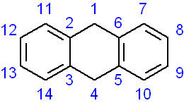
rotate C1 C4 C5 C6 C7 C8 C9 C10
the phenyl ring C5-C6-C7-C8-C9-C10 will be rigidly rotated around the axis C1-C4
shift_atom val
or
shift_atom atom1 atom2 atom3 …. val
To optimize the atomic parameters by applying shifts (up to val) on the atoms with respect to the centre of gravity of the fragment. The default val is 0.5. Add atom1, atom2, atom3,… to refine only some specific atoms.
randomize n
To randomize the internal and external DOFs and the atomic parameters (if refined). n is an optional parameters used as seed of random generator.
po H K L
Activate the March-Dollase preferred orientation correction. H K L are three integer numbers necessary to specify the direction of the preferred orientation
bvres atom1 valence [sigma wei]
Set bond valence restraint specifying the atom name and the expected oxidation state omitting the sign. The deviation from the expected value sigma and the weight of restraint wei can be optionally indicated. The default values for sigma and wei are 0.3 and 1, respectively. The special character * can be used to apply the same restraints to group of atoms of the same atom type.
E.g.
Apply the bond valence restraints on all gallium atoms. The expected formal valence of Ga1, Ga2, Ga3, Ga4 is 3.
bvres Ga1 3
bvres Ga2 3
bvres Ga3 3
bvres Ga4 3
the same directives can be written in a more synthetic way as
bvres Ga* 3
bvpar El1 El2 Ro B [rmin rmax]
For each pair of atom types El1 and El2 the program searches in the database the corresponding bond valence parameters ( and
and  ) and assign a bond windows, i.e. the range of distances between any two atoms that are to be considered as bonds. These range is defined in terms of minimum and maximum distance rmin and rmax. The table of bond valence parameters is written in the output file. Use this directive only if the bond valence parameters and the bond window assigned in default by the program should be modified.
The command %fragment followed by the name of a file can be used to import molecular starting model from external input file. The file extension must be mandatory specified to enable the program to identify the type of file. A complete list of the supported input file can be find in section Import of this document.
The command %fragment may also be associated with specific keywords to generate some predefined molecular fragments without the use of external files. In this case the general form of the command is: %fragment keyword optionl [option2] [option3]
The keyword must be followed by at least one option to define further details of the molecular fragment. All possible keywords are listed below.
- %fragment tetra AtC AtV [dist]
%fragment octa AtC AtV [dist]
%fragment square AtC AtV [dist]
%fragment cube AtC AtV [dist]
%fragment trigonal AtC AtV [dist]
%fragment prism_tetra AtC AtV [dist]
%fragment prism_trig AtC AtV [dist]
%fragment icosa AtC AtV [dist]
The keywords tetra, octa, square, cube, trigonal, prism_tetra, prism_trig, icosa can be used to generate polyhedra, respectively tetrahedron, octahedron, square planar molecular geometry, cube, trigonal planar molecular geometry, tetragonal prism, trigonal prism, icosahedron. The keyword must be followed by the atomic specie AtC in the center of the geometry and the second atomic specie AtV at the vertices of the geometry. Optionally you can specify the distance dist between the two atomic species. If dist is absent the distance will be assigned by accessing an internal database of average distances.
E.g., %fragment tetra Si O import a silicon-oxygen tetrahedron SiO4 with default distance Si-O of 1.645 . %fragment tetra Si O 1.597 also specifies a Si-O distance of 1.5972 Å. - %fragment atoms chem_formula
The keyword atoms allows you to import isolated atoms in asymmetric unit. The keyword must be followed by the list of atomic species and their number as a chemical formula. Examples of valid formula: [C3H5(OH)3]4, C 28 O 8 S 4 H 24.
E.g., %fragment atoms Pb import an isolated atom of Pb in random position. %fragment atoms (Sb2O3)2 import 4 Sb atoms and 6 O atoms in random positions. - %fragment smiles SMILES_string
The keyword smiles allows you to import molecule from an ASCII string written by using the SMILES notation. The following input file can be used to load the starting model by using the keyword smiles and solve the crystal structure of paracetamol.
%Structure paracetamol
%Job Paracetamol (C8H9NO2)
%Data
Cell 7.100 9.380 11.708 90.0 97.42 90.0
SpaceGroup p 21/n
Pattern paracetamol.xy
Wavelength 1.54056
%fragment smiles CC(=O)NC1=CC=C(C=C1)O
%sannel
The command %fragment can be repeated several times to import more than one molecules. Some examples are reported.
Input file for the structure solution of the creatine monohydrate
%Structure creatinem
%Job Creatine monohydrate (C4H9N3O2.H2O)
%Data
        Cell   12.506  5.046  12.169  90  108.88  90
        SpaceGroup P 21/c
        Pattern    creatinem.xy
        Wavelength 1.54056
%fragment creatine.cif
%fragment H2O.sdf
%sannel
The command %fragment was used to import the cif file of the creatine molecule (creatine.cif) and the sdf file of the water molecule (H2O.sdf). The cell parameters and space group reported in the creatine.cif were ignored and the creatine molecule was imported in the cell and space group indicated by the user in the input file by directive Cell and SpaceGroup.
Input file for structure solution of S-Ibuprofen containing two molecules of Ibuprofen in the asymmetric unit (Z’=2)
%Structure S-Ibuprofen (C13 H18 O2)
%Job Structure solution of S-Ibuprofen
%Data
        Cell  12.463  8.029  13.538  90  112.93  90
        SpaceGroup p 21
        Pattern    pd_0034.pow
        Wavelength 1.54056
%fragment Structure3D_CID_3672.sdf
%fragment Structure3D_CID_3672.sdf
%sannel
Two molecules of ibuprofen were imported using the file Structure3D_CID_3672.sdf downloaded from the PubChem database (https://pubchem.ncbi.nlm.nih.gov/compound/962#section=Top).
Input file for structure solution of lead(II) sulfate (PbSO4).
%structure pbso4
%job Lead(II) sulfate (PbSO4)
%data
pattern pbso4.dat
wave 1.54056
cell 6.95802 8.48024 5.39754 90 90 90
space p b n m
%fragment tetra S O
%fragment atoms Pb
%sannel
The command %fragment was used to import a SO4 tetrahedron and an isolated atom of Pb.
deletehydro
This directive can be used to delete hydrogen atoms from a model.
E.g.
%fragment my_molecule
deletehydro
All hydrogen atoms in my_molecule.mol will be deleted.
cut at1 at2
This directive can be used to delete a bond between two atoms, at1 and at2. It is useful when there is a need to break certain bonds, particularly in rings, to make the system more flexible.
E.g:
%fragment my_molecule.mol
cut C1 C2
The C1-C2 bond in my_molecule.mol will be deleted.
Altomare, A., Corriero, N., Cuocci, C., Moliterni, A., Rizzi, R. (2013). J. Appl. Cryst., 46,779-787.
Falcioni, M., Deem, MW. (1999).J. Chem. Phys.110, 1754-1766.
Favre-Nicolin, V. & Černý, R. (2002). J.Appl. Cryst.35, 734-743.
Feng, Z.J., Jia, R.R., Dong, C., Cao, S.X. & Zhang, J.C. (2010). J.Appl. Cryst.43, 179—180.
Wayne A. Hendrickson, Stereochemically restrained refinement of macromolecular structures, Methods in Enzymology, Academic Press, Volume 115, 1985, Pages 252-270.