- Basics
- Create input file for Simulated Annealing
- Molecular description
- Graphic Interface of Simulated Annealing
- Output of Simulated Annealing
- When Simulated Annealing fails
- The directives in Simulated Annealing
- Contact
Simulated Annealing (SA), as well as similar procedures like grid search, Monte Carlo, parallel tempering, genetic algorithm, etc., involves the generation of a random sequence of trial structures starting from an appropriate 3D model. The parameters defining the model are modified until a good match between calculated and observed structure factors is found. The information about chemical knowledge of molecules is actively used to reduce the number of parameters to be changed: bond distances and angles are usually known and kept fixed. Global parameters defining the orientation and the position of each fragment are varied during the procedure, together with internal parameters like torsion angles.
The dynamical occupancy correction for atoms lying on special positions and atoms sharing the same position in the crystal structure may be taken into account.
In the following images, the Simulated Annealing dialog, the Sir2019 window during the run and the solution menu are reported.
To get help click on ![]()
To start click on ![]()
To look at solutions use ![]()
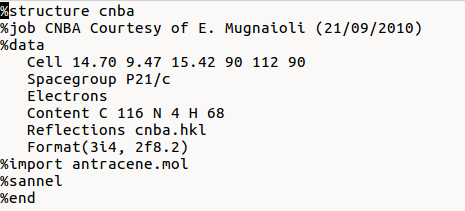
To run Sir2019 for structure solution by Simulated Annealing you need to create an input file (*.sir) using a text editor:
or using the program interface File > New.
In the tab “Solve” select “Simulated Annealing” in the frame Solving strategy and import the starting model. The following picture is an example of the interface for the crystal structure determination of the structure cnba using Simulated Annealing.
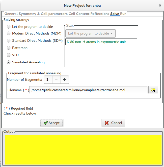
“%sannel” is a command to access to the simulated annealing graphical interface. “%import struct.mol” is the command to import the starting structural model for simulated annealing in MDL Molfile format (*.mol). This command can be repeated several times to import more than one fragment. Some other file type can be import in the same way: MOPAC file (*.mop), Tripos Sybyl file (*.mol2,*.ml2), C.I.F. file (*.cif), Protein Data Bank file (*.pdb), Sir fragment or Free Fractional Format (*.frac), XYZ format (*.xyz). Refer to openbabel wiki or http://www.ch.ic.ac.uk/chemime for information about common molecular file formats. Refer to http://en.wikipedia.org/wiki/Molecule_editor and http://www.ccp14.ac.uk/solution/2d_3d_model_builders/index.html for an exhaustive list of programs for building 3D starting models. Suggested free available programs for building 3D models are ACD/ChemSketch (windows), Avogadro (all platforms), Marvin (all platforms), ghemical (linux).
NIST Chemisty webbook and Drugbank are useful links to look up fragments.
Instead of command “%sannel”, you can access directly to the graphical interface from menu “Solve” > “Simulated Annealing”.
The required starting model can be described in terms of combination of scattering objects that are molecular fragments e.g., isolated atoms, molecules, coordination polyhedra. For each molecular fragment, the position may be defined by the fractional coordinates (x, y, z) of the center-of-mass or a predefined pivot atom, the orientation may be defined by rotation angles (θ, φ, χ) around a set of orthogonal axes, and the intramolecular geometry may be specified by a set of n variable torsion angles {τ1, τ2, …, τn}. These concepts may be extended to the case of two or more (identical or nonidentical) molecular fragments within the asymmetric unit (a.u.). In general bond lengths, bond angles and ring conformation are not considered as variables during the optimization procedure, but they should match as closely as possible that of the studied compound. One of the drawbacks of global optimization methods is to input an accurate 3D starting structural model of the a.u.
Starting model for direct-space method can be prepared by the following two strategies, or by a combination of both approaches.
1) The user is strongly advised to check for similar molecules in the Cambridge Structure Database (CSD) (organics & organometallics) or in the Inorganic Crystal Structure Database (ICSD) (inorganics, elements, minerals & intermetallics) or in the Crystallography Open Database (COD: http://www.crystallography.net/) or in the crystallographic literature. If a new structure is being studied, one can frequently find significant molecular parts of the structure in existing crystal structures. Molecular fragment found in database can be modified and optimized by quantum-chemistry package to finally generate the desired structure.
Some open chemistry database where look up molecules are:
- NIST Chemistry WebBook: http://webbook.nist.gov/chemistry/
- PubChem: https://pubchem.ncbi.nlm.nih.gov/
- Drugbank: http://www.drugbank.ca/
You can verify that the bond lengths have reasonable values using a tables of standard bond lengths available in Volume C of International Tables for X-Ray Crystallography.
2) Starting molecular model can be created by geometry optimization using quantum-chemistry package, e.g., MOPAC, Gaussian, Gamess, NWChem, etc. Nowadays this is usually done by building the molecule with an interactive builder in a graphical user interface, then optimizing it with forcefield method with the click of mouse. The resulting structure is then subjected to an ab initio, semi-empirical, or DFT calculations.
Some free available software that can be used to sketch molecules, optimize the geometry by forcefield method and create input file for the quantum-chemistry calculations are:
- Avogadro: http://avogadro.cc/wiki/Main_Page
- Gabedit: http://gabedit.sourceforge.net/
- ACD/ChemSketch: http://www.acdlabs.com/resources/freeware/chemsketch/
- MarvinSketch: https://www.chemaxon.com/products/marvin/marvinsketch/
The description of crystal structure is straightforward in the case of molecular organic crystals: isolated molecules with known chemical connectivity are packed together by weak intermolecular forces. Because the starting model should be a tridimensional representation of the a.u., is important to known how many molecules are contained in the a.u. (Z’). In case of molecular compounds the a.u. is usually a molecule or occasionally two or more molecules which differ from one another in orientation or conformation (Z’>1). When a molecule posses symmetry coincident with a crystallographic symmetry element, it may occupy a special position, and the a.u. will then be a half molecule or even some smaller fraction (Z’<1). Inorganic materials often consist of connected polyhedra and the topology of this connectivity is not generally known a priori and thus building a model of inorganic crystal structure for global optimization is often less straightforward and clear. Software provides tool to import some regular polyhedra or you can find the type of polyhedra you need from literature or from database. The choice of the number of each polyhedra to use must be made, talking into account how many atoms are expected per unit cell (volume of atom in the cell). These non‐molecular crystals usually crystallize with higher symmetries, and atoms often occupy special positions. At the same time it is necessary to take into account the possibility that polyhedra share atoms at the corners. The use of dynamical occupancy correction (DOC) is able to automatically correct the occupancy of atoms if they are close to a special position or in case of overlap between atoms of the same atomic type. DOC could be very useful when the exact composition of the studied compound is a priori not known exactly. Theoretically this means that it is possible to add more atoms than initially deemed necessary, expecting the DOC to artificially merge the excess atoms. It is also possible to solve structures putting into the cell independent atoms at random positions, but the observation/parameter ratio (‘observation’ here means the number of reflections) should be at least 8 or more depending on the quality of diffraction data.
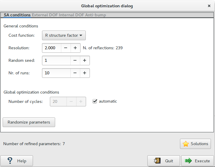
The dialog of Simulated Anneling in Sir2019 is composed by 4 pages (tabs).
The first page ‘SA conditions‘ contains the general settings of the Simulated Annealing algorithm:
Cost function: 2 cost functions can be selected: R structure factor (default cost function), R intensities.
Resolution: define the maximum resolution used by Simulated Annealing procedure. Usually the algorithm works well with data up to 2 Å resolution.
Random seed: select the value determining the sequence of random numbers used from the algorithm. When it is set to 0 the random seed will be calculated by the system clock.
Nr. of runs: select the number of Simulated Annealing (SA) runs. At the beginning of each run a new value of random seed is calculated.
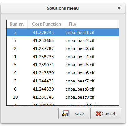
Solutions: browse the best solutions saved at the end of each run.
The second page ‘External DOF‘ contains information about the external degrees of freedom (DOF)
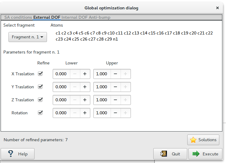
Select fragment: select the fragment and visualize the corresponding structure information.
Parameter for fragment: list of the external DOFs for the selected fragment. Check the parameters to refine, enter the lower and upper bounds of the parameters.
The third page ‘Internal DOF‘ contains information about the internal DOFs
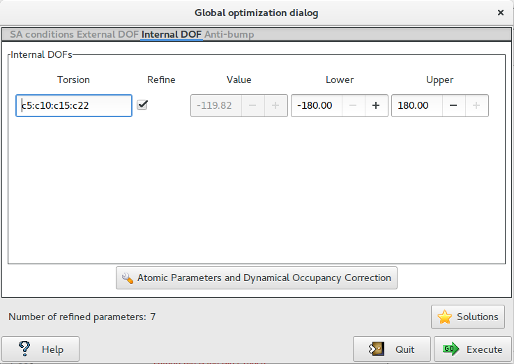
Internal DOFs: list of the torsions associated to each refinable internal DOF. Check the parameters to refine, enter the lower and upper bounds of parameters.
Dynamical Occupancy Correction: automatic detection of atoms in special position and atoms that share the same position. If this option is not active all refined atoms are considered in general position (default).
The “Atomic parameters and Dynamical Occupancy Correction” button ![]() give access to the following dialog
give access to the following dialog
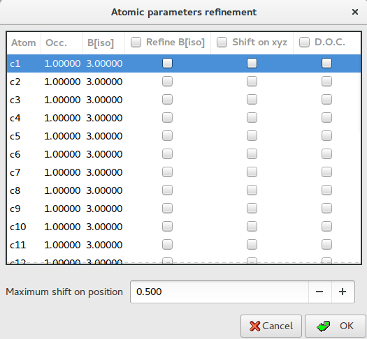
Thermal parameters: check the buttons on column ‘B[iso]‘ to refine the thermal parameters of atoms. Click on label ‘B[iso]‘ to select all checks in the column. If the thermal parameters are not indicated in the imported fragment file, the program assigns the default values of B=3.0 for non-hydrogen atoms and B=6.0 for hydrogen atoms. These default values can be changed editing the new values in the column. The refinement of the thermal parameters is discouraged because usually doesn’t improve the results.
X Y Z: check the buttons on column ‘Shift on xyz’ to refine the atom positions, in this case the fragment is not rigid but the atom positions are shifted respect to the barycentre. Click on label ‘Shift on syz’ to select all checks in the column. The positions refinement (x,y,z) is generally discouraged because can considerably increase the time to reach the global minimum.
Maximum shift on position: enter the value of the maximum shift of the atomic positions. 0.020 is the suggested value. Increasing this value the explored parameter space becomes wider so increasing the probability of falling into a local minimum.
Dynamical Occupancy Correction (DOC): automatic detection of atoms in special position and atoms that share the same position. If this option is not active all refined atoms are considered in general position (default). DOC will be applied only on the atoms selected in the column D.O.C., select all atoms if you don’t know exactly which atoms will fall into special positions. DOC slows down the computation time so it should be avoid if non special position or shared atoms are expected
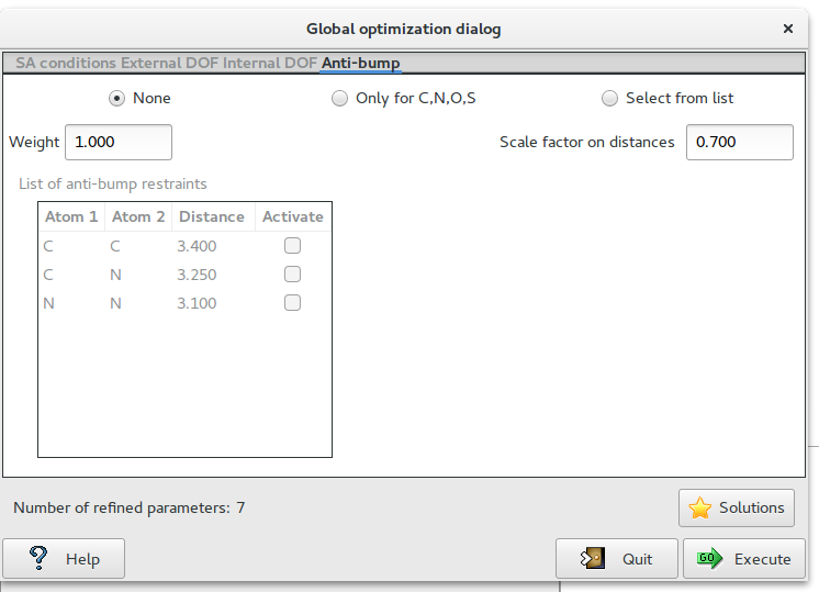
The fourth page ‘Anti-bump‘ contains information about the anti-bump restraints.
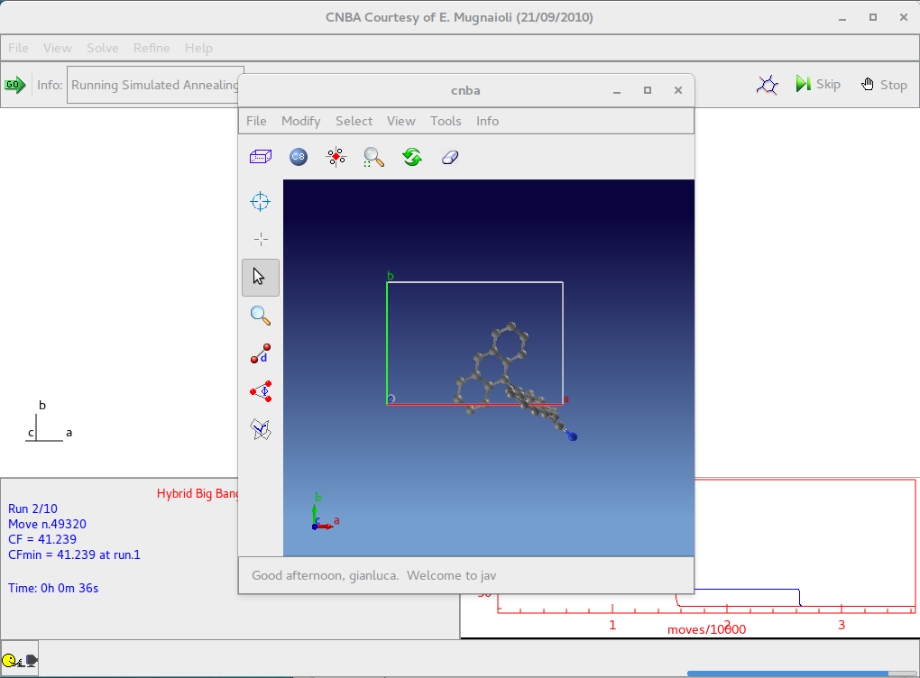
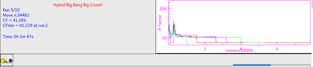
When simulated annealing is running the progress of structure solution is monitored and the user can examine the graph of the minimum values of cost function (CF) vs. the number of moves. The crystal packing is plotted in the JAV viewer.
The output file contains information on:
1) the starting structure
2) the volume per atom
2) the connectivity
3) the internal and external DOFs
4) the refined parameters by SA
5) the information about each SA run
6) the summary of all the SA runs
7) the selected structure
At the end of each run the structure coordinates are saved in CIF file with name created by project name with suffix _best1,_best2, … (e.g. cnba_best1.cif is the best solution, cnba_best2.cif is the second best solution, …). The order number in the name represents the position in the list of structures ordered according to the cost function.
If Simulated Annealing fails:
- Starting model is incorrect: bond distances and angle are not entirely accurate, number of building blocks is wrong. Improve your model with Cambridge Structural Database (CSD) or building packages (Avogadro, ChemSketch, ChemDraw, …). Check for the volume per atom in the output file (about 15-20 Å/atom).
- The assumption about thermal factors are invalid. Check thermal factors for similar structures.
- Space group and cell are not correct. Additionally, in many cases it may be necessary to carry out a series of independent calculations to test different potential space groups and/or unit cell choices.
- For complex structures the default SA conditions are not sufficient. Try with slower temperature reduction, increase the number of moves and/or runs.
Usually the user does not need to know the directives unless he is interested to run Simulated Annealing without interaction with the graphic interface. The list of directives is available here.
For suggestions and bugs contact corrado.cuocci@ic.cnr.it